
Is that lucky streak real - or did you just look hard enough?
A real question from the wild, worked the way a biostatistician would. The trap behind it is the one that also quietly wrecks subgroup results in clinical trials.
From the wild: r/AskStatistics
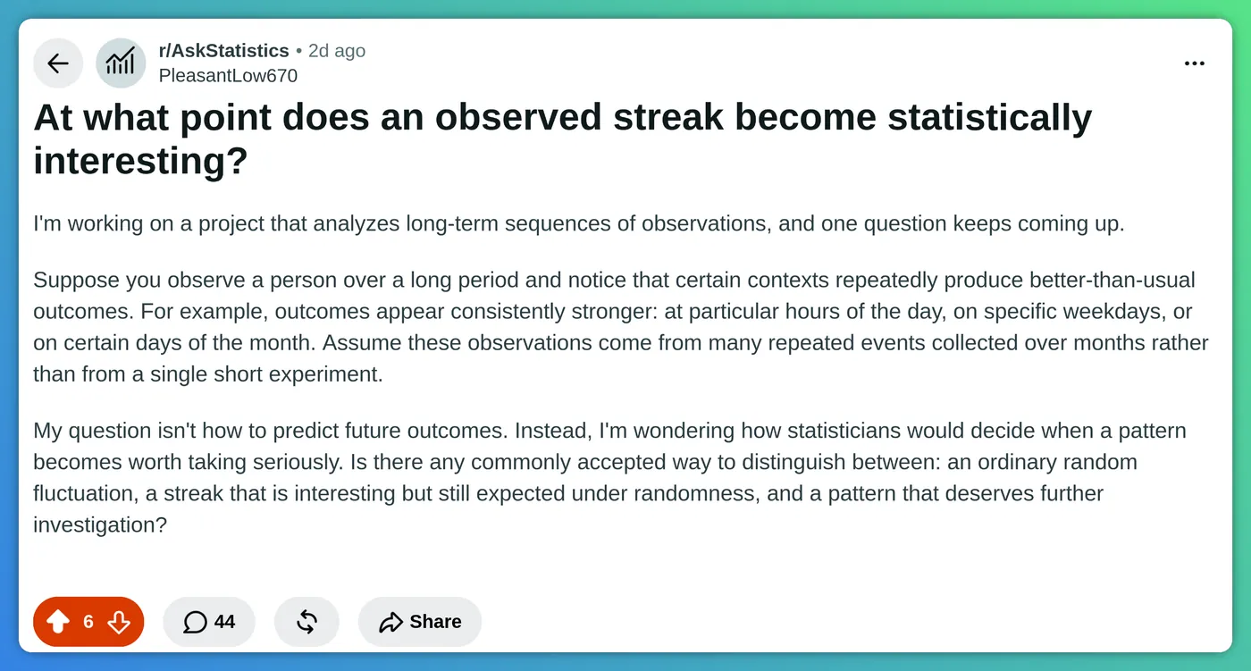
Suppose you observe a person over a long period and notice that certain contexts repeatedly produce better-than-usual outcomes - at particular hours of the day, on specific weekdays, or on certain days of the month, over months of repeated events. My question isn't how to predict future outcomes. It's how statisticians decide when a pattern becomes worth taking seriously. Is there a commonly accepted way to distinguish an ordinary random fluctuation, a streak that is interesting but still expected under randomness, and a pattern that deserves further investigation?
☝ Before you read on: how would you answer this? Pick the reply closest to yours - then see how it holds up.
The quick read
The question asks when the evidence for a lucky context gets strong enough. That's the wrong question. With this setup you're not measuring whether a pattern is real - you're measuring how hard you looked. Scanning dozens of time-contexts, re-checking as data pile up, and crowning the best one after the fact is a machine for turning pure noise into “significant” luck.
- Look-everywhere. 24 hours + 7 weekdays + 31 days of the month = 62 contexts tested at once. At the usual 5% bar, pure noise alone hands you about 3 “significant” ones.
- Peeking. Re-testing as data accumulate is guaranteed to eventually cross any fixed threshold, even when nothing is there.
- Pick-the-winner. Choosing the best context after seeing the data means it will disappoint next period - plain regression to the mean.
So the honest question is not “when is the evidence strong enough?” but “is my best context stronger than what chance would throw up across 62 tries - and does it hold up on fresh data?”
Why this fools careful people too
The instinct - “collect more data until the pattern is undeniable” - feels rigorous and is exactly backwards. More data does not rescue you here, because the problem isn't the sample size of any one context; it's the number of contexts and the freedom to pick the best.
Same shape in the clinic every day: many patients, many lab values, checked over and over. Watch enough dials long enough and some will alarm for no reason - it is part of how a sepsis alarm that cried wolf ended up ignored by the very clinicians it was built for.
What to actually do: a 5-step plan
This is the simplest disciplined approach. Each step is plain first, with the maths and numbers a click away.
1Count how many patterns you could have found
Before testing anything, list every context you scan - and include the ones you glanced at and dropped. Hours, weekdays, days of the month: 24 + 7 + 31 = 62. Look at combinations (“Friday evenings”) and you are into the hundreds.
The number that matters
Call it m, the number of tests. At a 5% threshold, the expected count of false alarms is m times 0.05. For m = 62 that is about 3 - so finding three “lucky” contexts is exactly what noise produces. Counting the tests you never formally ran (the garden of forking paths) is the hard, honest part.
2Give each context a score
For each context, turn the average outcome into a z-score: how many standard errors above “no effect” it sits. Under the null of no luck, every context's z behaves like a draw from a standard bell curve. Say your best context lands at z = 2.6 - a raw p-value near 0.005, which looks impressive against 0.05.
The formula
For a context with mean score x-bar over n observations and spread s:
More observations shrink the denominator, so the same real edge shows up as a bigger z. That is the grain of truth in “collect more data” - but it does nothing about the 62 looks in the next step.
Where the numbers come from: three worked examples
Three small datasets, three shapes of data - and the same recipe every time: (observed average − average expected under no luck), divided by the standard error.
For each dataset we walk the path an analyst would walk at the keyboard: look at a few raw rows, sanity-check the file as a whole, group by the context, then turn each group into one z. The highlighted rows are the numbers the rest of the page keeps reusing.
Example 1 - a continuous score with a known expectation. Six months of the asker's simulated-lottery log: 1,800 rows, one per play, with columns date, hour, weekday and score - the outcome already normalized against the game's known expectation, so “no luck” means an average score of 0, and single plays scatter with spread s = 1. Context to test: “Tuesdays”, which holds n = 260 plays averaging x-bar = +0.16. Standard error = s/√n = 1/√260 ≈ 0.062, so z = 0.16/0.062 ≈ 2.6 - the z we carry through this whole page.
What the log actually looks like - the first rows of the file:
| date | hour | weekday | score |
|---|---|---|---|
| 2026-01-05 | 09:00 | Mon | −0.42 |
| 2026-01-05 | 14:00 | Mon | +1.13 |
| 2026-01-06 | 10:00 | Tue | +0.77 |
| 2026-01-06 | 15:00 | Tue | −0.08 |
| 2026-01-07 | 11:00 | Wed | +0.31 |
| … 1,795 more rows | |||
Micro-EDA before any pattern hunting: the mean of all 1,800 scores is +0.004 with spread 1.00 - the normalization behaves, and a broken score column would show up right here. Now group by weekday and summarise each group: how many plays it holds, their average, and that average divided by its own standard error:
| weekday | n | mean | z |
|---|---|---|---|
| Mon | 258 | −0.03 | −0.5 |
| Tue | 260 | +0.16 | +2.6 |
| Wed | 255 | +0.05 | +0.8 |
| Thu | 259 | −0.11 | −1.8 |
| Fri | 254 | +0.02 | +0.3 |
| Sat | 257 | −0.07 | −1.1 |
| Sun | 257 | +0.01 | +0.2 |
Six weekdays hover where noise lives; Tuesday pokes out at z = 2.6. Repeat the same group-and-summarise for the 24 hours and the 31 days of the month, and you hold all 62 z's - the column that steps 3 to 5 will judge.
Example 2 - win/lose outcomes. A game where each try wins with a known probability of 20% - the expectation is known by design, as in the asker's lottery simulations. 2,100 rows: timestamp, hour, win (1 or 0). Context: “the 3pm hour”, with n = 150 tries and 41 wins - a rate of 27.3% against the expected 20%. For a proportion the standard error is √(p(1−p)/n) with p the expected rate: √(0.20 × 0.80/150) ≈ 0.033, so z = (0.273 − 0.200)/0.033 ≈ 2.2. Same recipe - only the standard-error formula changes with the data type.
The raw log:
| timestamp | hour | win |
|---|---|---|
| 2026-02-03 15:12 | 15 | 1 |
| 2026-02-03 18:40 | 18 | 0 |
| 2026-02-04 11:05 | 11 | 0 |
| … 2,097 more rows | ||
Micro-EDA: 424 wins out of 2,100 tries - an overall rate of 20.2%, sitting right on the designed 20%, so the game is fair overall and any luck must hide in the slices. Note the unequal group sizes: plays cluster in waking hours, so busy hours hold about 150 tries and early-morning ones far fewer - which is exactly why the summary keeps n visible. Group by hour:
| hour | n | wins | rate | z |
|---|---|---|---|---|
| 09:00 | 138 | 26 | 18.8% | −0.3 |
| 12:00 | 142 | 30 | 21.1% | +0.3 |
| 15:00 | 150 | 41 | 27.3% | +2.2 |
| 18:00 | 147 | 27 | 18.4% | −0.5 |
| 21:00 | 131 | 28 | 21.4% | +0.4 |
| … 19 more hours | ||||
Only 15:00 leaves the pack - and the rest of this page is about deciding whether even that is anything.
Example 3 - sparse subjective ratings. The asker's second stream: 400 evening self-assessments, columns date and rating - −1 (worse than usual), 0 (as expected), +1 (better). Here no external expectation exists, so “no luck” is the person's own long-run average - subtract it first; say the centered ratings scatter with s = 0.75. Context: “the 13th of the month” - only n = 13 evenings, but they average x-bar = +0.31, and it feels like “the 13th is my day”. Standard error = 0.75/√13 ≈ 0.21, so z = 0.31/0.21 ≈ 1.5. The lesson: rare contexts have tiny n, so even a big-looking average sits comfortably inside noise - and that is before the 62-contexts correction.
The raw log:
| date | rating |
|---|---|
| 2026-03-05 | +1 |
| 2026-03-06 | 0 |
| 2026-03-07 | −1 |
| … 397 more rows | |
Micro-EDA: the 400 ratings split into 118 × (−1), 172 × 0 and 110 × (+1) - overall mean −0.02, spread s = 0.75. No designed expectation exists here, so that −0.02 is the person's own baseline: subtract it from everything before comparing contexts, otherwise a generally gloomy or cheerful rater fakes a signal in every slice. Group by day of the month:
| day of month | n | centered mean | z |
|---|---|---|---|
| 3 | 13 | −0.12 | −0.6 |
| 8 | 14 | +0.06 | +0.3 |
| 13 | 13 | +0.31 | +1.5 |
| 21 | 13 | +0.17 | +0.8 |
| 27 | 13 | −0.23 | −1.1 |
| … 26 more days | |||
Look at what this table quietly teaches: with n around 13 per day, the centered means swing between −0.23 and +0.31 while nothing real is going on anywhere - single days of the month are simply that noisy. The 13th's +0.31 feels like a lot; z = 1.5 says a 13-evening average wanders that far routinely.
Whatever the shape of the data, the same three ingredients: an observed average, the average you would expect under no luck, and a standard error that shrinks like the square root of n. That z is what steps 3 to 5 judge.
The whole procedure in one line, runnable on any log: group rows by context; count n and average each group; subtract the no-luck average; divide by the standard error (s/√n for scores, √(p(1−p)/n) for win/lose) - and you hold one z per context. If your data can produce tables like the ones above, you can run every step on this page yourself.
3Simulate the ceiling of pure luck
This is the heart of it - and the playground below does it live. Shuffle which hour and day each outcome belongs to (this breaks any real time link but keeps the data's shape), recompute all 62 contexts, and record the best z. Repeat thousands of times, and you get the distribution of “the luckiest of 62 contexts under pure noise.” Compare your real best to it.
The numbers, and the quick shortcut
For 62 contexts, the best-of-62 z under pure noise has a median near 2.3 and a 95th percentile near 3.1. Your 2.6 sits around the 75th percentile - noise matches or beats it roughly one run in four. Not interesting. The “worth a look” line is about z = 3.1. Shortcut without simulating: Bonferroni asks each context to clear 0.05 divided by 62, about 0.0008 (z above 3.2) - your 2.6 fails. If you would rather screen many candidates than make one hard claim, control the false discovery rate (Benjamini-Hochberg) instead. Medical scale-up: genome studies test about a million sites and use a threshold of 5 in 100 million.
Is this a bootstrap?
A close cousin, but no. The bootstrap resamples your data with replacement to ask “how much would my estimate wobble in a fresh sample from the same world?” - it measures the uncertainty around a value. What step 3 does is a permutation test: shuffle the time labels without replacement to build the world where luck definitely does not exist, then see where your real result falls in it. And taking the best of all 62 contexts in every shuffled run is the classic max-T scheme (Westfall-Young) - it handles multiplicity more honestly than Bonferroni, because the shuffles automatically respect the overlap between contexts (the same play sits in both “Tuesday” and “3pm”), where Bonferroni over-corrects.
And yes - the verdict needs no bell-curve table at all: you simply check whether your real best lands in the top 5% tail of the shuffled distribution (one-sided, because “lucky” is a directional claim). One catch stops you from dropping the z-score entirely: contexts come in very different sizes, and raw averages are not comparable across them. Take the two contexts from step 2. “Tuesdays” holds n = 260 plays, so its average wobbles with a standard error of about 0.062 - under pure noise it stays roughly within ±0.12 of zero (two standard errors). “The 13th of the month” holds only n = 13 evenings, standard error about 0.21 - an average roughly 3.4 times noisier, which the same pure chance routinely swings out to ±0.4. Rank contexts by raw average and the rare ones win almost every shuffled run, simply because they are noisier - your 260-play Tuesdays can never out-wobble a 13-evening context, no matter how real their edge is. Dividing each average by its own standard error (that is all the z-score is) puts every context on one ruler: one z unit now costs the same amount of surprise everywhere, and the maximum becomes a fair contest. Any statistic with that property works - including each context's own permutation p-value (the min-p variant).
Full disclosure: the playground below draws independent bell-curve z's rather than shuffling a real dataset - the right simplification for a lesson. On your own data, the real permutation is strictly better: it inherits your data's odd distributions and the dependence between contexts for free.
4Confirm on data you didn't use to find it
The big one, and the line between “interesting” and “real.” The pattern you spotted is a hypothesis, not evidence. Freeze the surviving context as one pre-named claim, then test only that context on the second half of your history - or, better, on new observations going forward - at a plain 5%.
Why this fixes almost everything
At the confirmation stage there is no multiplicity - you test one thing you named in advance, so a plain 5% is honest again. This is also what defeats peeking and regression to the mean in one move: a fluke found by looking everywhere will not repeat on data it never touched. If it replicates, it earns further study; if it evaporates, it was noise all along. Pre-registering the hypothesis, or an N-of-1 design, formalises the same idea.
5Ask how big, not just whether
Report the size of the edge and its confidence interval, not only a p-value. Over months of data even a microscopic effect becomes “significant” - so significant and worth acting on are not the same thing.
Try it: the look-everywhere simulator
Set how many contexts you scan, how many observations each holds, and how strong your best one looks. The chart is 4,000 runs of pure noise - the distribution of the luckiest context when nothing real is going on. See where your result lands.
A subtlety worth noticing: push observations up and, with the average edge held fixed, the result rightly gets more impressive - a real effect can clear even the raised bar, given enough data. The catch is that a noise-born pattern won't hold its average: it melts toward zero as observations pile up. Prolonging the same exploration never settles it - which is why fresh data (step 4) is the decider.
The three buckets, answered
Two of those get built rather than promised in our Monte Carlo series - sequential designs, calibrated by simulation, where the very move this page runs - simulate the null, take the quantile of the maximum - comes back to fix the peeking problem for real.
Frequently asked
When does a streak become statistically significant?
There is no fixed amount of data that turns a streak into a real signal. If you scan many contexts (hours, weekdays, days of the month), pure chance guarantees a few will look significant. Significance for a hand-picked context is meaningless until you correct for how many patterns you tested and confirm the winner on data you did not use to find it.
What is the multiple comparisons problem?
When you run many tests at once, each has its own chance of a false positive. Testing 62 contexts at the 5 percent level produces about three significant results from pure noise. Corrections such as Bonferroni or the false discovery rate keep the overall false-positive rate under control.
How do you tell a real pattern from random noise?
Count how many patterns you tested, shrink your threshold or simulate the best result pure noise would produce across that many tries, then confirm any surviving pattern on fresh data. A pattern that clears the noise ceiling and replicates out of sample deserves investigation; one that does not is regression to the mean.
Sources
- ISIS-2 Collaborative Group, The Lancet, 1988 - the trial whose authors ran the astrological subgroup analysis on purpose.
- r/AskStatistics - the original thread this case is built on.
- xkcd 882, “Significant” - the green-jelly-bean version of the same trap.
Traps like this one are a whole section of Stat Exam Pro - exam-style questions with worked answers, in English and French.
Get it on iPhone